Numeric Javascript

Reference card for the numeric module

Function	Description

`abs`	Absolute value
`acos`	Arc-cosine
`add`	Pointwise sum x+y
`addeq`	Pointwise sum x+=y
`all`	All the components of x are true
`and`	Pointwise x && y
`andeq`	Pointwise x &= y
`any`	One or more of the components of x are true
`asin`	Arc-sine
`atan`	Arc-tangeant
`atan2`	Arc-tangeant (two parameters)
`band`	Pointwise x & y
`bench`	Benchmarking routine
`bnot`	Binary negation ~x
`bor`	Binary or x\|y
`bxor`	Binary xor x^y
`ccsDim`	Dimensions of sparse matrix
`ccsDot`	Sparse matrix-matrix product
`ccsFull`	Convert sparse to full
`ccsGather`	Gather entries of sparse matrix
`ccsGetBlock`	Get rows/columns of sparse matrix
`ccsLUP`	Compute LUP decomposition of sparse matrix
`ccsLUPSolve`	Solve Ax=b using LUP decomp
`ccsScatter`	Scatter entries of sparse matrix
`ccsSparse`	Convert from full to sparse
`ccsTSolve`	Solve upper/lower triangular system
`ccs<op>`	Supported ops include: add/div/mul/geq/etc...
`cLU`	Coordinate matrix LU decomposition
`cLUsolve`	Coordinate matrix LU solve
`cdelsq`	Coordinate matrix Laplacian
`cdotMV`	Coordinate matrix-vector product
`ceil`	Pointwise Math.ceil(x)
`cgrid`	Coordinate grid for cdelsq
`clone`	Deep copy of Array
`cos`	Pointwise Math.cos(x)
`det`	Determinant
`diag`	Create diagonal matrix
`dim`	Get Array dimensions
`div`	Pointwise x/y
`diveq`	Pointwise x/=y
`dopri`	Numerical integration of ODE using Dormand-Prince RK method. Returns an object Dopri.
`Dopri.at`	Evaluate the ODE solution at a point

Function	Description

`dot`	Matrix-Matrix, Matrix-Vector and Vector-Matrix product
`eig`	Eigenvalues and eigenvectors
`epsilon`	2.220446049250313e-16
`eq`	Pointwise comparison x === y
`exp`	Pointwise Math.exp(x)
`floor`	Poinwise Math.floor(x)
`geq`	Pointwise x>=y
`getBlock`	Extract a block from a matrix
`getDiag`	Get the diagonal of a matrix
`gt`	Pointwise x>y
`identity`	Identity matrix
`imageURL`	Encode a matrix as an image URL
`inv`	Matrix inverse
`isFinite`	Pointwise isFinite(x)
`isNaN`	Pointwise isNaN(x)
`largeArray`	Don't prettyPrint Arrays larger than this
`leq`	Pointwise x<=y
`linspace`	Generate evenly spaced values
`log`	Pointwise Math.log(x)
`lshift`	Pointwise x<<y
`lshifteq`	Pointwise x<<=y
`lt`	Pointwise x<y
`LU`	Dense LU decomposition
`LUsolve`	Dense LU solve
`mapreduce`	Make a pointwise map-reduce function
`mod`	Pointwise x%y
`modeq`	Pointwise x%=y
`mul`	Pointwise x*y
`neg`	Pointwise -x
`neq`	Pointwise x!==y
`norm2`	Square root of the sum of the square of the entries of x
`norm2Squared`	Sum of squares of entries of x
`norminf`	Largest modulus entry of x
`not`	Pointwise logical negation !x
`or`	Pointwise logical or x\|\|y
`oreq`	Pointwise x\|=y
`parseCSV`	Parse a CSV file into an Array
`parseDate`	Pointwise parseDate(x)
`parseFloat`	Pointwise parseFloat(x)
`pointwise`	Create a pointwise function
`pow`	Pointwise Math.pow(x)
`precision`	Number of digits to prettyPrint
`prettyPrint`	Pretty-prints x
`random`	Create an Array of random numbers
`rep`	Create an Array by duplicating values

Function	Description

`round`	Pointwise Math.round(x)
`rrshift`	Pointwise x>>>y
`rrshifteq`	Pointwise x>>>=y
`rshift`	Pointwise x>>y
`rshifteq`	Pointwise x>>=y
`same`	x and y are entrywise identical
`seedrandom`	The seedrandom module
`setBlock`	Set a block of a matrix
`sin`	Pointwise Math.sin(x)
`solve`	Solve Ax=b
`solveLP`	Solve a linear programming problem
`solveQP`	Solve a quadratic programming problem
`spline`	Create a Spline object
`Spline.at`	Evaluate the Spline at a point
`Spline.diff`	Differentiate the Spline
`Spline.roots`	Find all the roots of the Spline
`sqrt`	Pointwise Math.sqrt(x)
`sub`	Pointwise x-y
`subeq`	Pointwise x-=y
`sum`	Sum all the entries of x
`svd`	Singular value decomposition
`t`	Create a tensor type T (may be complex-valued)
`T.<numericfun>`	Supported <numericfun> are: abs, add, cos, diag, div, dot, exp, getBlock, getDiag, inv, log, mul, neg, norm2, setBlock, sin, sub, transpose
`T.conj`	Pointwise complex conjugate
`T.fft`	Fast Fourier transform
`T.get`	Read an entry
`T.getRow`	Get a row
`T.getRows`	Get a range of rows
`T.ifft`	Inverse FFT
`T.reciprocal`	Pointwise 1/z
`T.set`	Set an entry
`T.setRow`	Set a row
`T.setRows`	Set a range of rows
`T.transjugate`	The conjugate-transpose of a matrix
`tan`	Pointwise Math.tan(x)
`tensor`	Tensor product ret[i][j] = x[i]*y[j]
`toCSV`	Make a CSV file
`transpose`	Matrix transpose
`uncmin`	Unconstrained optimization
`version`	Version string for the numeric library
`xor`	Pointwise x^y
`xoreq`	Pointwise x^=y

Numerical analysis in Javascript

Numeric Javascript is library that provides many useful functions for numerical calculations, particularly for linear algebra (vectors and matrices). You can create vectors and matrices and multiply them:

IN> A = [[1,2,3],[4,5,6]];
OUT> [[1,2,3],
      [4,5,6]]
IN> x = [7,8,9]
OUT> [7,8,9]
IN> numeric.dot(A,x);
OUT> [50,122]

The example shown above can be executed in the Javascript Workshop or at any Javascript prompt. The Workshop provides plotting capabilities:

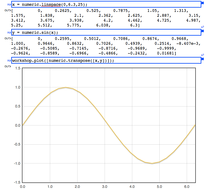
The function workshop.plot() is essentially the flot plotting command.

The numeric library provides functions that implement most of the usual Javascript operators for vectors and matrices:

IN> x = [7,8,9];
    y = [10,1,2];
    numeric['+'](x,y)
OUT> [17,9,11]
IN> numeric['>'](x,y)
OUT> [false,true,true]

These operators can also be called with plain Javascript function names:

IN> numeric.add([7,8,9],[10,1,2])
OUT> [17,9,11]

You can also use these operators with three or more parameters:

IN> numeric.add([1,2],[3,4],[5,6],[7,8])
OUT> [16,20]

The function numeric.inv() can be used to compute the inverse of an invertible matrix:

IN> A = [[1,2,3],[4,5,6],[7,1,9]]
OUT> [[1,2,3],
      [4,5,6],
      [7,1,9]]
IN> Ainv = numeric.inv(A);
OUT> [[-0.9286,0.3571,0.07143],
      [-0.1429,0.2857,-0.1429],
      [0.7381,-0.3095,0.07143]]

The function numeric.prettyPrint() is used to print most of the examples in this documentation. It formats objects, arrays and numbers so that they can be understood easily. All output is automatically formatted using numeric.prettyPrint() when in the Workshop. In order to present the information clearly and succintly, the function numeric.prettyPrint() lays out matrices so that all the numbers align. Furthermore, numbers are given approximately using the numeric.precision variable:

IN> numeric.precision = 10; x = 3.141592653589793
OUT> 3.141592654
IN> numeric.precision = 4; x
OUT> 3.142

The default precision is 4 digits. In addition to printing approximate numbers, the function numeric.prettyPrint() will replace large arrays with the string ...Large Array...:

IN> numeric.identity(100)
OUT> ...Large Array...

By default, this happens with the Array's length is more than 50. This can be controlled by setting the variable numeric.largeArray to an appropriate value:

IN> numeric.largeArray = 2; A = numeric.identity(4)
OUT> ...Large Array...
IN> numeric.largeArray = 50; A
OUT> [[1,0,0,0],
      [0,1,0,0],
      [0,0,1,0],
      [0,0,0,1]]

In particular, if you want to print all Arrays regardless of size, set numeric.largeArray = Infinity.

Math Object functions

The Math object functions have also been adapted to work on Arrays as follows:

IN> numeric.exp([1,2]);
OUT> [2.718,7.389]
IN> numeric.exp([[1,2],[3,4]])
OUT> [[2.718, 7.389],
      [20.09, 54.6]]
IN> numeric.abs([-2,3])
OUT> [2,3]
IN> numeric.acos([0.1,0.2])
OUT> [1.471,1.369]
IN> numeric.asin([0.1,0.2])
OUT> [0.1002,0.2014]
IN> numeric.atan([1,2])
OUT> [0.7854,1.107]
IN> numeric.atan2([1,2],[3,4])
OUT> [0.3218,0.4636]
IN> numeric.ceil([-2.2,3.3])
OUT> [-2,4]
IN> numeric.floor([-2.2,3.3])
OUT> [-3,3]
IN> numeric.log([1,2])
OUT> [0,0.6931]
IN> numeric.pow([2,3],[0.25,7.1])
OUT> [1.189,2441]
IN> numeric.round([-2.2,3.3])
OUT> [-2,3]
IN> numeric.sin([1,2])
OUT> [0.8415,0.9093]
IN> numeric.sqrt([1,2])
OUT> [1,1.414]
IN> numeric.tan([1,2])
OUT> [1.557,-2.185]

Utility functions

The function numeric.dim() allows you to compute the dimensions of an Array.

IN> numeric.dim([1,2])
OUT> [2]
IN> numeric.dim([[1,2,3],[4,5,6]])
OUT> [2,3]

You can perform a deep comparison of Arrays using numeric.same():

IN> numeric.same([1,2],[1,2])
OUT> true
IN> numeric.same([1,2],[1,2,3])
OUT> false
IN> numeric.same([1,2],[[1],[2]])
OUT> false
IN> numeric.same([[1,2],[3,4]],[[1,2],[3,4]])
OUT> true
IN> numeric.same([[1,2],[3,4]],[[1,2],[3,5]])
OUT> false
IN> numeric.same([[1,2],[2,4]],[[1,2],[3,4]])
OUT> false

You can create a multidimensional Array from a given value using numeric.rep()

IN> numeric.rep([3],5)
OUT> [5,5,5]
IN> numeric.rep([2,3],0)
OUT> [[0,0,0],
      [0,0,0]]

You can loop over Arrays as you normally would. However, in order to quickly generate optimized loops, the numeric library provides a few efficient loop-generation mechanisms. For example, the numeric.mapreduce() function can be used to make a function that computes the sum of all the entries of an Array.

IN> sum = numeric.mapreduce('accum += xi','0'); sum([1,2,3])
OUT> 6
IN> sum([[1,2,3],[4,5,6]])
OUT> 21

The functions numeric.any() and numeric.all() allow you to check whether any or all entries of an Array are boolean true values.

IN> numeric.any([false,true])
OUT> true
IN> numeric.any([[0,0,3.14],[0,false,0]])
OUT> true
IN> numeric.any([0,0,false])
OUT> false
IN> numeric.all([false,true])
OUT> false
IN> numeric.all([[1,4,3.14],["no",true,-1]])
OUT> true
IN> numeric.all([0,0,false])
OUT> false

You can create a diagonal matrix using numeric.diag()

IN> numeric.diag([1,2,3])
OUT> [[1,0,0],
      [0,2,0],
      [0,0,3]]

The function numeric.identity() returns the identity matrix.

IN> numeric.identity(3)
OUT> [[1,0,0],
      [0,1,0],
      [0,0,1]]

Random Arrays can also be created:

IN> numeric.random([2,3])
OUT> [[0.05303,0.1537,0.7280],
      [0.3839,0.08818,0.6316]]

You can generate a vector of evenly spaced values:

IN> numeric.linspace(1,5);
OUT> [1,2,3,4,5]
IN> numeric.linspace(1,3,5);
OUT> [1,1.5,2,2.5,3]

Arithmetic operations

The standard arithmetic operations have been vectorized:

IN> numeric.addVV([1,2],[3,4])
OUT> [4,6]
IN> numeric.addVS([1,2],3)
OUT> [4,5]

There are also polymorphic functions:

IN> numeric.add(1,[2,3])
OUT> [3,4]
IN> numeric.add([1,2,3],[4,5,6])
OUT> [5,7,9]

The other arithmetic operations are available:

IN> numeric.sub([1,2],[3,4])
OUT> [-2,-2]
IN> numeric.mul([1,2],[3,4])
OUT> [3,8]
IN> numeric.div([1,2],[3,4])
OUT> [0.3333,0.5]

The in-place operators (such as +=) are also available:

IN> v = [1,2,3,4]; numeric.addeq(v,3); v
OUT> [4,5,6,7]
IN> numeric.subeq([1,2,3],[5,3,1])
OUT> [-4,-1,2]

Unary operators:

IN> numeric.neg([1,-2,3])
OUT> [-1,2,-3]
IN> numeric.isFinite([10,NaN,Infinity])
OUT> [true,false,false]
IN> numeric.isNaN([10,NaN,Infinity])
OUT> [false,true,false]

Linear algebra

Matrix products are implemented in the functions numeric.dotVV() numeric.dotVM() numeric.dotMV() numeric.dotMM():

IN> numeric.dotVV([1,2],[3,4])
OUT> 11
IN> numeric.dotVM([1,2],[[3,4],[5,6]])
OUT> [13,16]
IN> numeric.dotMV([[1,2],[3,4]],[5,6])
OUT> [17,39]
IN> numeric.dotMMbig([[1,2],[3,4]],[[5,6],[7,8]])
OUT> [[19,22],
      [43,50]]
IN> numeric.dotMMsmall([[1,2],[3,4]],[[5,6],[7,8]])
OUT> [[19,22],
      [43,50]]
IN> numeric.dot([1,2,3,4,5,6,7,8,9],[1,2,3,4,5,6,7,8,9])
OUT> 285

The function numeric.dot() is "polymorphic" and selects the appropriate Matrix product:

IN> numeric.dot([1,2,3],[4,5,6])
OUT> 32
IN> numeric.dot([[1,2,3],[4,5,6]],[7,8,9])
OUT> [50,122]

Solving the linear problem Ax=b (Dan Huang):

IN> numeric.solve([[1,2],[3,4]],[17,39])
OUT> [5,6]

The algorithm is based on the LU decomposition:

IN> LU = numeric.LU([[1,2],[3,4]])
OUT> {LU:[[3     ,4     ],
          [0.3333,0.6667]],
       P:[1,1]}
IN> numeric.LUsolve(LU,[17,39])
OUT> [5,6]

The determinant:

IN> numeric.det([[1,2],[3,4]]);
OUT> -2
IN> numeric.det([[6,8,4,2,8,5],[3,5,2,4,9,2],[7,6,8,3,4,5],[5,5,2,8,1,6],[3,2,2,4,2,2],[8,3,2,2,4,1]]);
OUT> -1404

The matrix inverse:

IN> numeric.inv([[1,2],[3,4]])
OUT> [[   -2,    1],
      [  1.5, -0.5]]

The transpose:

IN> numeric.transpose([[1,2,3],[4,5,6]])
OUT> [[1,4],
      [2,5],
      [3,6]]
IN> numeric.transpose([[1,2,3,4,5,6,7,8,9,10,11,12]])
OUT> [[ 1],
      [ 2],
      [ 3],
      [ 4],
      [ 5],
      [ 6],
      [ 7],
      [ 8],
      [ 9],
      [10],
      [11],
      [12]]

You can compute the 2-norm of an Array, which is the square root of the sum of the squares of the entries.

IN> numeric.norm2([1,2])
OUT> 2.236

Computing the tensor product of two vectors:

IN> numeric.tensor([1,2],[3,4,5])
OUT> [[3,4,5],
      [6,8,10]]

Data manipulation

There are also some data manipulation functions. You can parse dates:

IN> numeric.parseDate(['1/13/2013','2001-5-9, 9:31']);
OUT> [1.358e12,9.894e11]

Parse floating point quantities:

IN> numeric.parseFloat(['12','0.1'])
OUT> [12,0.1]

Parse CSV files:

IN> numeric.parseCSV('a,b,c\n1,2.3,.3\n4e6,-5.3e-8,6.28e+4')
OUT> [[     "a",     "b",     "c"],
      [       1,     2.3,     0.3],
      [     4e6, -5.3e-8,   62800]]
IN> numeric.toCSV([[1.23456789123,2],[3,4]])
OUT> "1.23456789123,2
     3,4
     "

You can also fetch a URL (a thin wrapper around XMLHttpRequest):

IN> numeric.getURL('tools/helloworld.txt').responseText
OUT> "Hello, world!"

Complex linear algebra

You can also manipulate complex numbers:

IN> z = new numeric.T(3,4);
OUT> {x: 3, y: 4}
IN> z.add(5)
OUT> {x: 8, y: 4}
IN> w = new numeric.T(2,8);
OUT> {x: 2, y: 8}
IN> z.add(w)
OUT> {x: 5, y: 12}
IN> z.mul(w)
OUT> {x: -26, y: 32}
IN> z.div(w)
OUT> {x:0.5588,y:-0.2353}
IN> z.sub(w)
OUT> {x:1, y:-4}

Complex vectors and matrices can also be handled:

IN> z = new numeric.T([1,2],[3,4]);
OUT> {x: [1,2], y: [3,4]}
IN> z.abs()
OUT> {x:[3.162,4.472],y:}
IN> z.conj()
OUT> {x:[1,2],y:[-3,-4]}
IN> z.norm2()
OUT> 5.477
IN> z.exp()
OUT> {x:[-2.691,-4.83],y:[0.3836,-5.592]}
IN> z.cos()
OUT> {x:[-1.528,-2.459],y:[0.1658,-2.745]}
IN> z.sin()
OUT> {x:[0.2178,-2.847],y:[1.163,2.371]}
IN> z.log()
OUT> {x:[1.151,1.498],y:[1.249,1.107]}

Complex matrices:

IN> A = new numeric.T([[1,2],[3,4]],[[0,1],[2,-1]]);
OUT> {x:[[1, 2],
         [3, 4]],
      y:[[0, 1],
         [2,-1]]}
IN> A.inv();
OUT> {x:[[0.125,0.125],
         [  0.25,    0]],
      y:[[   0.5,-0.25],
         [-0.375,0.125]]}
IN> A.inv().dot(A)
OUT> {x:[[1,         0],
         [0,         1]],
      y:[[0,-2.776e-17],
         [0,         0]]}
IN> A.get([1,1])
OUT> {x: 4, y: -1}
IN> A.transpose()
OUT> { x: [[1, 3],
           [2, 4]],
       y: [[0, 2],
           [1,-1]] }
IN> A.transjugate()
OUT> { x: [[ 1, 3],
           [ 2, 4]],
       y: [[ 0,-2],
           [-1, 1]] }
IN> numeric.T.rep([2,2],new numeric.T(2,3));
OUT> { x: [[2,2],
           [2,2]],
       y: [[3,3],
           [3,3]] }

Eigenvalues

Eigenvalues:

IN> A = [[1,2,5],[3,5,-1],[7,-3,5]];
OUT> [[ 1,  2,  5],
      [ 3,  5, -1],
      [ 7, -3,  5]]
IN> B = numeric.eig(A);
OUT> {lambda:{x:[-4.284,9.027,6.257],y:},
      E:{x:[[ 0.7131,-0.5543,0.4019],
            [-0.2987,-0.2131,0.9139],
            [-0.6342,-0.8046,0.057 ]],
         y:}}
IN> C = B.E.dot(numeric.T.diag(B.lambda)).dot(B.E.inv());
OUT> {x: [[ 1,  2,  5],
          [ 3,  5, -1],
          [ 7, -3,  5]],
      y: }

Note that eigenvalues and eigenvectors are returned as complex numbers (type numeric.T). This is because eigenvalues are often complex even when the matrix is real.

Singular value decomposition (Shanti Rao)

Shanti Rao kindly emailed me an implementation of the Golub and Reisch algorithm:

IN> A=[[ 22, 10,  2,  3,  7],
       [ 14,  7, 10,  0,  8],
       [ -1, 13, -1,-11,  3],
       [ -3, -2, 13, -2,  4],
       [  9,  8,  1, -2,  4],
       [  9,  1, -7,  5, -1],
       [  2, -6,  6,  5,  1],
       [  4,  5,  0, -2,  2]];
    numeric.svd(A);
OUT> {U:
[[    -0.7071,    -0.1581,     0.1768,     0.2494,     0.4625],
 [    -0.5303,    -0.1581,    -0.3536,     0.1556,    -0.4984],
 [    -0.1768,     0.7906,    -0.1768,    -0.1546,     0.3967],
 [ -1.506e-17,    -0.1581,    -0.7071,    -0.3277,        0.1],
 [    -0.3536,     0.1581,  1.954e-15,   -0.07265,    -0.2084],
 [    -0.1768,    -0.1581,     0.5303,    -0.5726,   -0.05555],
 [ -7.109e-18,    -0.4743,    -0.1768,    -0.3142,     0.4959],
 [    -0.1768,     0.1581,  1.915e-15,     -0.592,    -0.2791]],
S:
[      35.33,         20,       19.6,          0,          0],
V:
[[    -0.8006,    -0.3162,     0.2887,    -0.4191,          0],
 [    -0.4804,     0.6325,  7.768e-15,     0.4405,     0.4185],
 [    -0.1601,    -0.3162,     -0.866,     -0.052,     0.3488],
 [  4.684e-17,    -0.6325,     0.2887,     0.6761,     0.2442],
 [    -0.3203,  3.594e-15,    -0.2887,      0.413,    -0.8022]]}

Sparse linear algebra

Sparse matrices are matrices that have a lot of zeroes. In numeric, sparse matrices are stored in the "compressed column storage" ordering. Example:

IN> A = [[1,2,0],
         [0,3,0],
         [2,0,5]];
    SA = numeric.ccsSparse(A);
OUT> [[0,2,4,5],
      [0,2,0,1,2],
      [1,2,2,3,5]]

The relation between A and its sparse representation SA is:

    A[i][SA[1][k]] = SA[2][k] with SA[0][i] ≤ k < SA[0][i+1]

In other words, SA[2] stores the nonzero entries of A; SA[1] stores the row numbers and SA[0] stores the offsets of the columns. See I. DUFF, R. GRIMES, AND J. LEWIS, Sparse matrix test problems, ACM Trans. Math. Soft., 15 (1989), pp. 1-14.

IN> A = numeric.ccsSparse([[ 3, 5, 8,10, 8],
                          [ 7,10, 3, 5, 3],
                          [ 6, 3, 5, 1, 8],
                          [ 2, 6, 7, 1, 2],
                          [ 1, 2, 9, 3, 9]]);
OUT> [[0,5,10,15,20,25],
      [0,1,2,3,4,0,1,2,3,4,0,1,2,3,4,0,1,2,3,4,0,1,2,3,4],
      [3,7,6,2,1,5,10,3,6,2,8,3,5,7,9,10,5,1,1,3,8,3,8,2,9]]
IN> numeric.ccsFull(A);
OUT> [[ 3, 5, 8,10, 8],
      [ 7,10, 3, 5, 3],
      [ 6, 3, 5, 1, 8],
      [ 2, 6, 7, 1, 2],
      [ 1, 2, 9, 3, 9]]
IN> numeric.ccsDot(numeric.ccsSparse([[1,2,3],[4,5,6]]),numeric.ccsSparse([[7,8],[9,10],[11,12]]))
OUT> [[0,2,4],
      [0,1,0,1],
      [58,139,64,154]]
IN> M = [[0,1,3,6],[0,0,1,0,1,2],[3,-1,2,3,-2,4]];
    b = [9,3,2];
    x = numeric.ccsTSolve(M,b);
OUT> [3.167,2,0.5]
IN> numeric.ccsDot(M,[[0,3],[0,1,2],x])
OUT> [[0,3],[0,1,2],[9,3,2]]

We provide an LU=PA decomposition:

IN> A = [[0,5,10,15,20,25],
         [0,1,2,3,4,0,1,2,3,4,0,1,2,3,4,0,1,2,3,4,0,1,2,3,4],
         [3,7,6,2,1,5,10,3,6,2,8,3,5,7,9,10,5,1,1,3,8,3,8,2,9]];
    LUP = numeric.ccsLUP(A);
OUT> {L:[[0,5,9,12,14,15],
         [0,2,4,1,3,1,3,4,2,2,4,3,3,4,4],
         [1,0.1429,0.2857,0.8571,0.4286,1,-0.1282,-0.5641,-0.1026,1,0.8517,0.7965,1,-0.67,1]],
      U:[[0,1,3,6,10,15],
         [0,0,1,0,1,2,0,1,2,3,0,1,2,3,4],
         [7,10,-5.571,3,2.429,8.821,5,-3.286,1.949,5.884,3,5.429,9.128,0.1395,-3.476]],
      P:[1,2,4,0,3],
      Pinv:[3,0,1,4,2]}
IN> numeric.ccsFull(numeric.ccsDot(LUP.L,LUP.U))
OUT> [[ 7,10, 3, 5, 3],
      [ 6, 3, 5, 1, 8],
      [ 1, 2, 9, 3, 9],
      [ 3, 5, 8,10, 8],
      [ 2, 6, 7, 1, 2]]
IN> x = numeric.ccsLUPSolve(LUP,[96,63,82,51,89])
OUT> [3,1,4,1,5]
IN> X = numeric.trunc(numeric.ccsFull(numeric.ccsLUPSolve(LUP,A)),1e-15); // Solve LUX = PA
OUT> [[1,0,0,0,0],
      [0,1,0,0,0],
      [0,0,1,0,0],
      [0,0,0,1,0],
      [0,0,0,0,1]]
IN> numeric.ccsLUP(A,0.4).P;
OUT> [0,2,1,3,4]

The LUP decomposition uses partial pivoting and has an optional thresholding argument. With a threshold of 0.4, the pivots are [0,2,1,3,4] (only rows 1 and 2 have been exchanged) instead of the "full partial pivoting" order above which was [1,2,4,0,3]. Threshold=0 gives no pivoting and threshold=1 gives normal partial pivoting. Note that a small or zero threshold can result in numerical instabilities and is normally used when the matrix A is already in some order that minimizes fill-in. We also support arithmetic on CCS matrices:

IN> A = numeric.ccsSparse([[1,2,0],[0,3,0],[0,0,5]]);
    B = numeric.ccsSparse([[2,9,0],[0,4,0],[-2,0,0]]);
    numeric.ccsadd(A,B);
OUT> [[0,2,4,5],
      [0,2,0,1,2],
      [3,-2,11,7,5]]

We also have scatter/gather functions

IN> X = [[0,0,1,1,2,2],[0,1,1,2,2,3],[1,2,3,4,5,6]];
    SX = numeric.ccsScatter(X);
OUT> [[0,1,3,5,6],
      [0,0,1,1,2,2],
      [1,2,3,4,5,6]]
IN> numeric.ccsGather(SX)
OUT> [[0,0,1,1,2,2],[0,1,1,2,2,3],[1,2,3,4,5,6]]

Coordinate matrices

We also provide a banded matrix implementation using the coordinate encoding.

LU decomposition:

IN> lu = numeric.cLU([[0,0,1,1,1,2,2],[0,1,0,1,2,1,2],[2,-1,-1,2,-1,-1,2]])
OUT> {U:[[    0,    0,    1,      1,  2   ],
         [    0,    1,    1,      2,  2   ],
         [    2,   -1,  1.5,     -1, 1.333]],
      L:[[    0,    1,    1,      2,  2   ],
         [    0,    0,    1,      1,  2   ],
         [    1, -0.5,    1,-0.6667,  1   ]]}
IN> numeric.cLUsolve(lu,[5,-8,13])
OUT> [3,1,7]

Note that numeric.cLU() does not have any pivoting.

Solving PDEs

The functions numeric.cgrid() and numeric.cdelsq() can be used to obtain a numerical Laplacian for a domain.

IN> g = numeric.cgrid(5)
OUT>
[[-1,-1,-1,-1,-1],
 [-1, 0, 1, 2,-1],
 [-1, 3, 4, 5,-1],
 [-1, 6, 7, 8,-1],
 [-1,-1,-1,-1,-1]]
IN> coordL = numeric.cdelsq(g)
OUT>
[[ 0, 0, 0, 1, 1, 1, 1, 2, 2, 2, 3, 3, 3, 3, 4, 4, 4, 4, 4, 5, 5, 5, 5, 6, 6, 6, 7, 7, 7, 7, 8, 8, 8],
 [ 1, 3, 0, 0, 2, 4, 1, 1, 5, 2, 0, 4, 6, 3, 1, 3, 5, 7, 4, 2, 4, 8, 5, 3, 7, 6, 4, 6, 8, 7, 5, 7, 8],
 [-1,-1, 4,-1,-1,-1, 4,-1,-1, 4,-1,-1,-1, 4,-1,-1,-1,-1, 4,-1,-1,-1, 4,-1,-1, 4,-1,-1,-1, 4,-1,-1, 4]]
IN> L = numeric.sscatter(coordL); // Just to see what it looks like
OUT>
[[          4,         -1,           ,         -1],
 [         -1,          4,         -1,           ,         -1],
 [           ,         -1,          4,           ,           ,         -1],
 [         -1,           ,           ,          4,         -1,           ,         -1],
 [           ,         -1,           ,         -1,          4,         -1,           ,         -1],
 [           ,           ,         -1,           ,         -1,          4,           ,           ,         -1],
 [           ,           ,           ,         -1,           ,           ,          4,         -1],
 [           ,           ,           ,           ,         -1,           ,         -1,          4,         -1],
 [           ,           ,           ,           ,           ,         -1,           ,         -1,          4]]
IN> lu = numeric.cLU(coordL); x = numeric.cLUsolve(lu,[1,1,1,1,1,1,1,1,1]);
OUT> [0.6875,0.875,0.6875,0.875,1.125,0.875,0.6875,0.875,0.6875]
IN> numeric.cdotMV(coordL,x)
OUT> [1,1,1,1,1,1,1,1,1]
IN> G = numeric.rep([5,5],0); for(i=0;i<5;i++) for(j=0;j<5;j++) if(g[i][j]>=0) G[i][j] = x[g[i][j]]; G
OUT>
[[ 0     , 0     , 0     , 0     , 0     ],
 [ 0     , 0.6875, 0.875 , 0.6875, 0     ],
 [ 0     , 0.875 , 1.125 , 0.875 , 0     ],
 [ 0     , 0.6875, 0.875 , 0.6875, 0     ],
 [ 0     , 0     , 0     , 0     , 0     ]]
IN> workshop.html('<img src="'+numeric.imageURL(numeric.mul([G,G,G],200))+'" width=100 />');
OUT>

You can also work on an L-shaped or arbitrary-shape domain:

IN> numeric.cgrid(6,'L')
OUT>
[[-1,-1,-1,-1,-1,-1],
 [-1, 0, 1,-1,-1,-1],
 [-1, 2, 3,-1,-1,-1],
 [-1, 4, 5, 6, 7,-1],
 [-1, 8, 9,10,11,-1],
 [-1,-1,-1,-1,-1,-1]]
IN> numeric.cgrid(5,function(i,j) { return i!==2 || j!==2; })
OUT>
[[-1,-1,-1,-1,-1],
 [-1, 0, 1, 2,-1],
 [-1, 3,-1, 4,-1],
 [-1, 5, 6, 7,-1],
 [-1,-1,-1,-1,-1]]

Cubic splines

You can do some (natural) cubic spline interpolation:

IN> numeric.spline([1,2,3,4,5],[1,2,1,3,2]).at(numeric.linspace(1,5,10))
OUT> [ 1, 1.731, 2.039, 1.604, 1.019, 1.294, 2.364, 3.085, 2.82, 2]

For clamped splines:

IN> numeric.spline([1,2,3,4,5],[1,2,1,3,2],0,0).at(numeric.linspace(1,5,10))
OUT> [ 1, 1.435, 1.98, 1.669, 1.034, 1.316, 2.442, 3.017, 2.482, 2]

For periodic splines:

IN> numeric.spline([1,2,3,4],[0.8415,0.04718,-0.8887,0.8415],'periodic').at(numeric.linspace(1,4,10))
OUT> [ 0.8415, 0.9024, 0.5788, 0.04718, -0.5106, -0.8919, -0.8887, -0.3918, 0.3131, 0.8415]

Vector splines:

IN> numeric.spline([1,2,3],[[0,1],[1,0],[0,1]]).at(1.78)
OUT> [0.9327,0.06728]

Spline differentiation:

IN> xs = [0,1,2,3]; numeric.spline(xs,numeric.sin(xs)).diff().at(1.5)
OUT> 0.07302

Find all the roots:

IN> xs = numeric.linspace(0,30,31); ys = numeric.sin(xs); s = numeric.spline(xs,ys).roots();
OUT> [0, 3.142, 6.284, 9.425, 12.57, 15.71, 18.85, 21.99, 25.13, 28.27]

Fast Fourier Transforms

FFT and IFFT on numeric.T objects:

IN> z = (new numeric.T([1,2,3,4,5],[6,7,8,9,10])).fft()
OUT> {x:[15,-5.941,-3.312,-1.688, 0.941],
      y:[40, 0.941,-1.688,-3.312,-5.941]}
IN> z.ifft()
OUT> {x:[1,2,3,4,5],
      y:[6,7,8,9,10]}

Quadratic Programming (Alberto Santini)

The Quadratic Programming function numeric.solveQP() is based on Alberto Santini's quadprog, which is itself a port of the corresponding R routines.

IN> numeric.solveQP([[1,0,0],[0,1,0],[0,0,1]],[0,5,0],[[-4,2,0],[-3,1,-2],[0,0,1]],[-8,2,0]);
OUT> { solution:              [0.4762,1.048,2.095],
       value:                 [-2.381],
       unconstrained_solution:[     0,    5,    0],
       iterations:            [     3,    0],
       iact:                  [     3,    2,    0],
       message:               "" }

Unconstrained optimization

To minimize a function f(x) we provide the function numeric.uncmin(f,x0) where x0 is a starting point for the optimization. Here are some demos from from Moré et al., 1981:

IN> sqr = function(x) { return x*x; };
    numeric.uncmin(function(x) { return sqr(10*(x[1]-x[0]*x[0])) + sqr(1-x[0]); },[-1.2,1]).solution
OUT> [1,1]
IN> f = function(x) { return sqr(-13+x[0]+((5-x[1])*x[1]-2)*x[1])+sqr(-29+x[0]+((x[1]+1)*x[1]-14)*x[1]); };
    x0 = numeric.uncmin(f,[0.5,-2]).solution
OUT> [11.41,-0.8968]
IN> f = function(x) { return sqr(1e4*x[0]*x[1]-1)+sqr(Math.exp(-x[0])+Math.exp(-x[1])-1.0001); };
    x0 = numeric.uncmin(f,[0,1]).solution
OUT> [1.098e-5,9.106]
IN> f = function(x) { return sqr(x[0]-1e6)+sqr(x[1]-2e-6)+sqr(x[0]*x[1]-2)};
    x0 = numeric.uncmin(f,[0,1]).solution
OUT> [1e6,2e-6]
IN> f = function(x) {
       return sqr(1.5-x[0]*(1-x[1]))+sqr(2.25-x[0]*(1-x[1]*x[1]))+sqr(2.625-x[0]*(1-x[1]*x[1]*x[1]));
    };
    x0 = numeric.uncmin(f,[1,1]).solution
OUT> [3,0.5]
IN> f = function(x) {
        var ret = 0,i;
        for(i=1;i<=10;i++) ret+=sqr(2+2*i-Math.exp(i*x[0])-Math.exp(i*x[1]));
         return ret;
    };
    x0 = numeric.uncmin(f,[0.3,0.4]).solution
OUT> [0.2578,0.2578]
IN> y = [0.14,0.18,0.22,0.25,0.29,0.32,0.35,0.39,0.37,0.58,0.73,0.96,1.34,2.10,4.39];
    f = function(x) {
        var ret = 0,i;
        for(i=1;i<=15;i++) ret+=sqr(y[i-1]-(x[0]+i/((16-i)*x[1]+Math.min(i,16-i)*x[2])));
        return ret;
    };
    x0 = numeric.uncmin(f,[1,1,1]).solution
OUT> [0.08241,1.133,2.344]
IN> y = [0.0009,0.0044,0.0175,0.0540,0.1295,0.2420,0.3521,0.3989,0.3521,0.2420,0.1295,0.0540,0.0175,0.0044,0.0009];
    f = function(x) {
        var ret = 0,i;
        for(i=1;i<=15;i++)
        ret+=sqr(x[0]*Math.exp(-x[1]*sqr((8-i)/2-x[2])/2)-y[i-1]);
        return ret;
    };
    x0 = numeric.div(numeric.round(numeric.mul(numeric.uncmin(f,[1,1,1]).solution,1000)),1000)
OUT> [0.399,1,0]
IN> f = function(x) { return sqr(x[0]+10*x[1])+5*sqr(x[2]-x[3])+sqr(sqr(x[1]-2*x[2]))+10*sqr(x[0]-x[3]); };
    x0 = numeric.div(numeric.round(numeric.mul(numeric.uncmin(f,[3,-1,0,1]).solution,1e5)),1e5)
OUT> [0,0,0,0]
IN> f = function(x) {
        return (sqr(10*(x[1]-x[0]*x[0]))+sqr(1-x[0])+
                90*sqr(x[3]-x[2]*x[2])+sqr(1-x[2])+
                10*sqr(x[1]+x[3]-2)+0.1*sqr(x[1]-x[3])); };
    x0 = numeric.uncmin(f,[-3,-1,-3,-1]).solution
OUT> [1,1,1,1]
IN> y = [0.1957,0.1947,0.1735,0.1600,0.0844,0.0627,0.0456,0.0342,0.0323,0.0235,0.0246];
    u = [4,2,1,0.5,0.25,0.167,0.125,0.1,0.0833,0.0714,0.0625];
    f = function(x) {
        var ret=0, i;
        for(i=0;i<11;++i) ret += sqr(y[i]-x[0]*(u[i]*u[i]+u[i]*x[1])/(u[i]*u[i]+u[i]*x[2]+x[3]));
        return ret;
    };
    x0 = numeric.uncmin(f,[0.25,0.39,0.415,0.39]).solution
OUT> [     0.1928,     0.1913,     0.1231,     0.1361]
IN> y = [0.844,0.908,0.932,0.936,0.925,0.908,0.881,0.850,0.818,0.784,0.751,0.718,
         0.685,0.658,0.628,0.603,0.580,0.558,0.538,0.522,0.506,0.490,0.478,0.467,
         0.457,0.448,0.438,0.431,0.424,0.420,0.414,0.411,0.406];
    f = function(x) {
        var ret=0, i;
        for(i=0;i<33;++i) ret += sqr(y[i]-(x[0]+x[1]*Math.exp(-10*i*x[3])+x[2]*Math.exp(-10*i*x[4])));
        return ret;
    };
    x0 = numeric.uncmin(f,[0.5,1.5,-1,0.01,0.02]).solution
OUT> [     0.3754,      1.936,     -1.465,    0.01287,    0.02212]
IN> f = function(x) {
        var ret=0, i,ti,yi,exp=Math.exp;
        for(i=1;i<=13;++i) {
            ti = 0.1*i;
            yi = exp(-ti)-5*exp(-10*ti)+3*exp(-4*ti);
            ret += sqr(x[2]*exp(-ti*x[0])-x[3]*exp(-ti*x[1])+x[5]*exp(-ti*x[4])-yi);
        }
        return ret;
    };
    x0 = numeric.uncmin(f,[1,2,1,1,1,1],1e-14).solution;
    f(x0)<1e-20;
OUT> true

There are optional parameters to numeric.uncmin(f,x0,tol,gradient,maxit,callback). The iteration stops when the gradient or step size is less than the optional parameter tol. The gradient() parameter is a function that computes the gradient of f(). If it is not provided, a numerical gradient is used. The iteration stops when maxit iterations have been performed. The optional callback() parameter, if provided, is called at each step:

IN> z = [];
    cb = function(i,x,f,g,H) { z.push({i:i, x:x, f:f, g:g, H:H }); };
    x0 = numeric.uncmin(function(x) { return Math.cos(2*x[0]); },
                        [1],1e-10,
                        function(x) { return [-2*Math.sin(2*x[0])]; },
                        100,cb);
OUT> {solution:    [1.571],
      f:           -1,
      gradient:    [2.242e-11],
      invHessian:  [[0.25]],
      iterations:  6,
      message:     "Newton step smaller than tol"}
IN> z
OUT> [{i:0, x:[1    ], f:-0.4161, g: [-1.819   ]  , H:[[1     ]] },
      {i:2, x:[1.909], f:-0.7795, g: [ 1.253   ]  , H:[[0.296 ]] },
      {i:3, x:[1.538], f:-0.9979, g: [-0.1296  ]  , H:[[0.2683]] },
      {i:4, x:[1.573], f:-1     , g: [ 9.392e-3]  , H:[[0.2502]] },
      {i:5, x:[1.571], f:-1     , g: [-6.105e-6]  , H:[[0.25  ]] },
      {i:6, x:[1.571], f:-1     , g: [ 2.242e-11] , H:[[0.25  ]] }]

Linear programming

Linear programming is available:

IN> x = numeric.solveLP([1,1],                   /* minimize [1,1]*x                */
                        [[-1,0],[0,-1],[-1,-2]], /* matrix of inequalities          */
                        [0,0,-3]                 /* right-hand-side of inequalities */
                        );
    numeric.trunc(x.solution,1e-12);
OUT> [0,1.5]

The function numeric.solveLP(c,A,b) minimizes dot(c,x) subject to dot(A,x) <= b. The algorithm used is very basic. For alpha>0, define the ``barrier function'' f0 = dot(c,x) - alpha*sum(log(b-A*x)). The function numeric.solveLP calls numeric.uncmin on f0 for smaller and smaller values of alpha. This is a basic ``interior point method''. We also handle infeasible problems:

IN> numeric.solveLP([1,1],[[1,0],[0,1],[-1,-1]],[-1,-1,-1])
OUT> { solution: NaN, message: "Infeasible", iterations: 5 }

Unbounded problems:

IN> numeric.solveLP([1,1],[[1,0],[0,1]],[0,0]).message;
OUT> "Unbounded"

With an equality constraint:

IN> numeric.solveLP([1,2,3],                      /* minimize [1,2,3]*x                */
                    [[-1,0,0],[0,-1,0],[0,0,-1]], /* matrix A of inequality constraint */
                    [0,0,0],                      /* RHS b of inequality constraint    */
                    [[1,1,1]],                    /* matrix Aeq of equality constraint */
                    [3]                           /* vector beq of equality constraint */
                    );
OUT> { solution:[3,1.685e-16,4.559e-19], message:"", iterations:12 }

Solving ODEs

The function numeric.dopri() is an implementation of the Dormand-Prince-Runge-Kutta integrator with adaptive time-stepping:

IN> sol = numeric.dopri(0,1,1,function(t,y) { return y; })
OUT> { x:    [     0,   0.1, 0.1522, 0.361, 0.5792, 0.7843, 0.9813,     1],
       y:    [     1, 1.105,  1.164, 1.435,  1.785,  2.191,  2.668, 2.718],
       f:    [     1, 1.105,  1.164, 1.435,  1.785,  2.191,  2.668, 2.718],
       ymid: [ 1.051, 1.134,  1.293,   1.6,  1.977,  2.418,  2.693],
       iterations:8,
       events:,
       message:""}
IN> sol.at([0.3,0.7])
OUT> [1.35,2.014]

The return value sol contains the x and y values of the solution. If you need to know the value of the solution between the given x values, use the function sol.at(), which uses the extra information contained in sol.ymid and sol.f to produce approximations between these points. The integrator is also able to handle vector equations. This is a harmonic oscillator:

IN> sol = numeric.dopri(0,10,[3,0],function (x,y) { return [y[1],-y[0]]; });
    sol.at([0,0.5*Math.PI,Math.PI,1.5*Math.PI,2*Math.PI])
OUT> [[         3,         0],
      [ -9.534e-8,        -3],
      [        -3,  2.768e-7],
      [   3.63e-7,         3],
      [         3, -3.065e-7]]

Van der Pol:

IN> numeric.dopri(0,20,[2,0],function(t,y) { return [y[1], (1-y[0]*y[0])*y[1]-y[0]]; }).at([18,19,20])
OUT> [[ -1.208,   0.9916],
      [ 0.4258,    2.535],
      [  2.008, -0.04251]]

You can also specify a tolerance, a maximum number of iterations and an event function. The integration stops if the event function goes from negative to positive.

IN> sol = numeric.dopri(0,2,1,function (x,y) { return y; },1e-8,100,function (x,y) { return y-1.3; });
OUT> { x:          [     0, 0.0181, 0.09051, 0.1822,  0.2624],
       y:          [     1,  1.018,   1.095,    1.2,     1.3],
       f:          [     1,  1.018,   1.095,    1.2,     1.3],
       ymid:       [ 1.009,  1.056,   1.146,  1.249],
       iterations: 5,
       events:     true,
       message:    "" }

Note that at x=0.1822, the event function value was -0.1001 while at x=0.2673, the event value was 6.433e-3. The integrator thus terminated at x=0.2673 instead of continuing until the end of the integration interval.

Events can also be vector-valued:

IN> sol = numeric.dopri(0,2,1,
                        function(x,y) { return y; },
                        undefined,50,
                        function(x,y) { return [y-1.5,Math.sin(y-1.5)]; });
OUT> { x:          [    0,   0.2, 0.4055],
       y:          [    1, 1.221,    1.5],
       f:          [    1, 1.221,    1.5],
       ymid:       [1.105, 1.354],
       iterations: 2,
       events:     [true,true],
       message:    ""}

Seedrandom (David Bau)

The object numeric.seedrandom is based on David Bau's seedrandom.js. This small library can be used to create better pseudorandom numbers than Math.random() which can furthermore be "seeded".

IN> numeric.seedrandom.seedrandom(3); numeric.seedrandom.random()
OUT> 0.7569
IN> numeric.seedrandom.random()
OUT> 0.6139
IN> numeric.seedrandom.seedrandom(3); numeric.seedrandom.random()
OUT> 0.7569

For performance reasons, numeric.random() uses the default Math.random(). If you want to use the seedrandom version, just do Math.random = numeric.seedrandom.random. Note that this may slightly decrease the performance of all Math operations.